|
Denosing
Using Wavelets and
Projections onto the L1-Ball
L1-ball
denoising software provides
examples of
denoising using projection onto the epigraph of L1-ball
(PES-L1).
Description of each file is given in the related mfile. Moreover,
you can find
complete explanation of the PES-L1 algorithm and the codes in the given
pdf below. Please feel free to contact us if you had any question.
Denoising using Projection
onto Epigraph
Set of L1-ball (PES-L1):
Considering
the following signal:
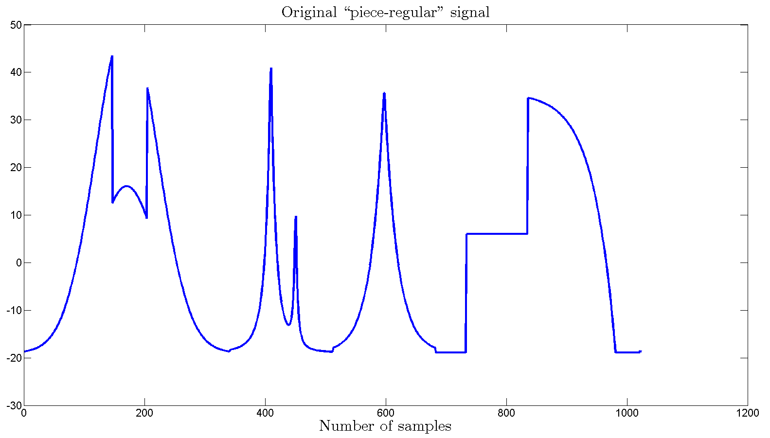
Fig.
1
This
signal is corrupted with additive, i.i.d. Gaussian noise with zero mean
(ξ [n]) as x[n] = v[n] + ξ[n], which v[n] is the original
discrete-time signal and x[n] is the noisy version of v[n],which has
standard deviation equal to 10% of the maximum amplitude of the
original signal, which is shown below:
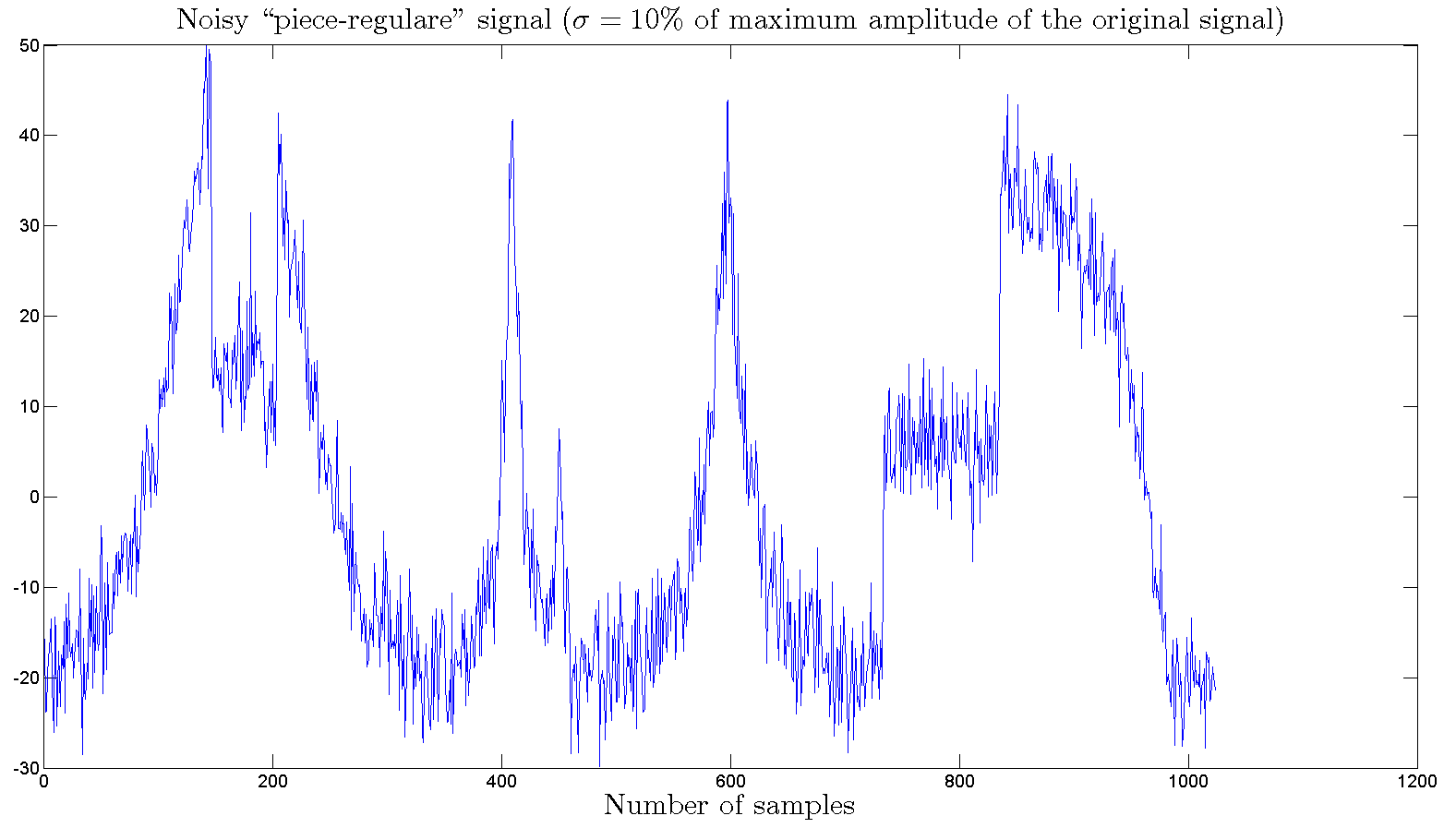
Fig.
2
PES-L1
using pyramidal structure:
PES-L1 ball
denoising is applied according to the followoing block-diagram:
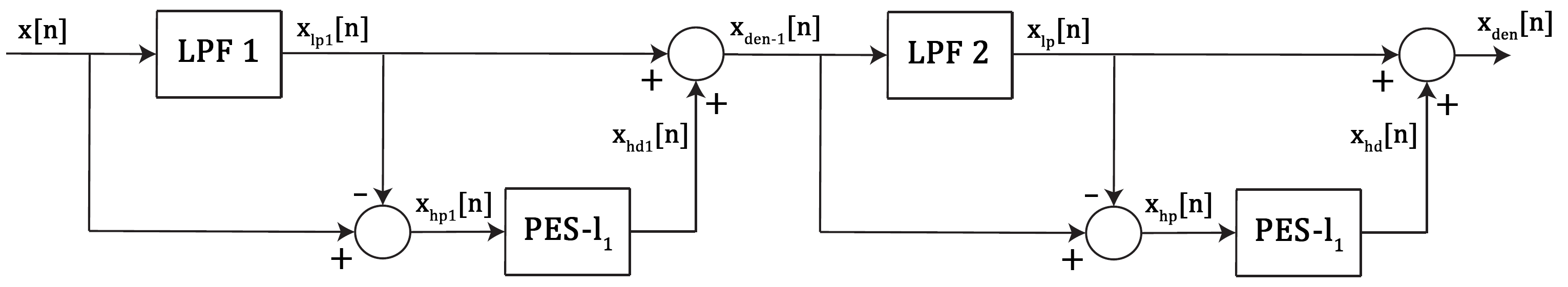
Fig.
3
The
noisy signal is low-pass filtered with cut-off frequency for
"piece-regular" signal and the output xlp[n]is
subtracted from the noisy signal to
obtain the high-pass signal xhp[n]as
shown in Fig. 3. The signal is projected onto the epigraph of L1-ball
and xhd[n]is
obtained. Projection onto the Epigraph Set of L1-ball (PES-L1), removes
the noise by soft-thresholding. The denoised signal xden[n]is
reconstructed by adding xhd[n]and xlp[n]as
shown in Fig. 3. Since the soft-thresholding is a nonlinear operation,
it may be advantages to iterate or circulate the signal several times
in the pyramidal structure as in wavelet denoising. A low-pass filter
with cut-off is
used in pyramidal structure.
And
the
resulting denoised signal, using this code PES_L1_Pyramid_Denoising,
is as follows:
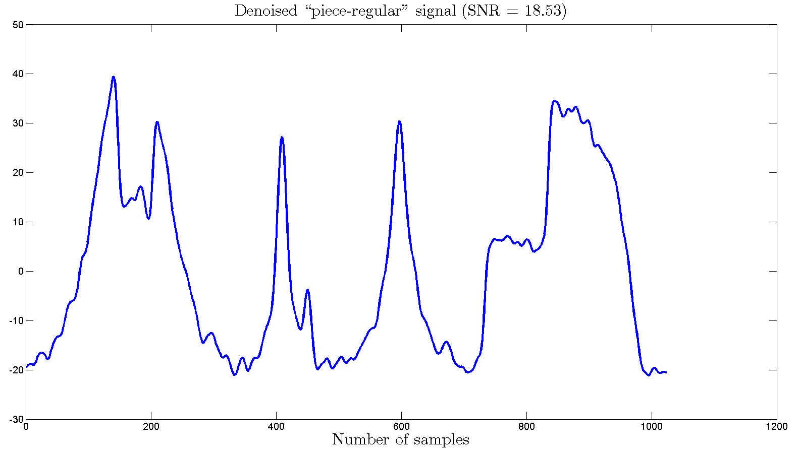
Fig.
4
PES-L1
using wavelet decomposition:
In
denoising using PES-L1 with wavelet decomposition the It is possible to
use the Fourier transform of the noisy signal to estimate the bandwidth
of the signal. Once the bandwidth ω0of
the original signal is approximately determined it can be used to
estimate the number of wavelet transform levels and the bandwidth of
the low-band signal xL.
In an -level
wavelet decomposition the low-band signal xLapproximately
comes from the frequency
band of the signal .
Therefore, must
be greater than ω0so
that the actual signal components are not soft-thresholded. Only
wavelet subsignals wLwL-1w1which
come from frequency bands , ,
..., ,
respectively, should be soft-thresholded in denoising. For example, in
Fig. 5,
the magnitude of Fourier transform ofis
shown for "piece-regular" signal defined in MATLAB. This signal is
corrupted by white Gaussian noise with of
the maximum amplitude of the original signal. For this signal a level
wavelet decomposition is suitable because Fourier transform magnitude
approaches to the noise floor level after ω0.
It is also a good practice to allow a margin for signal harmonics.
Therefore, L=3 (ω0)
is selected as the number of wavelet decomposition levels.
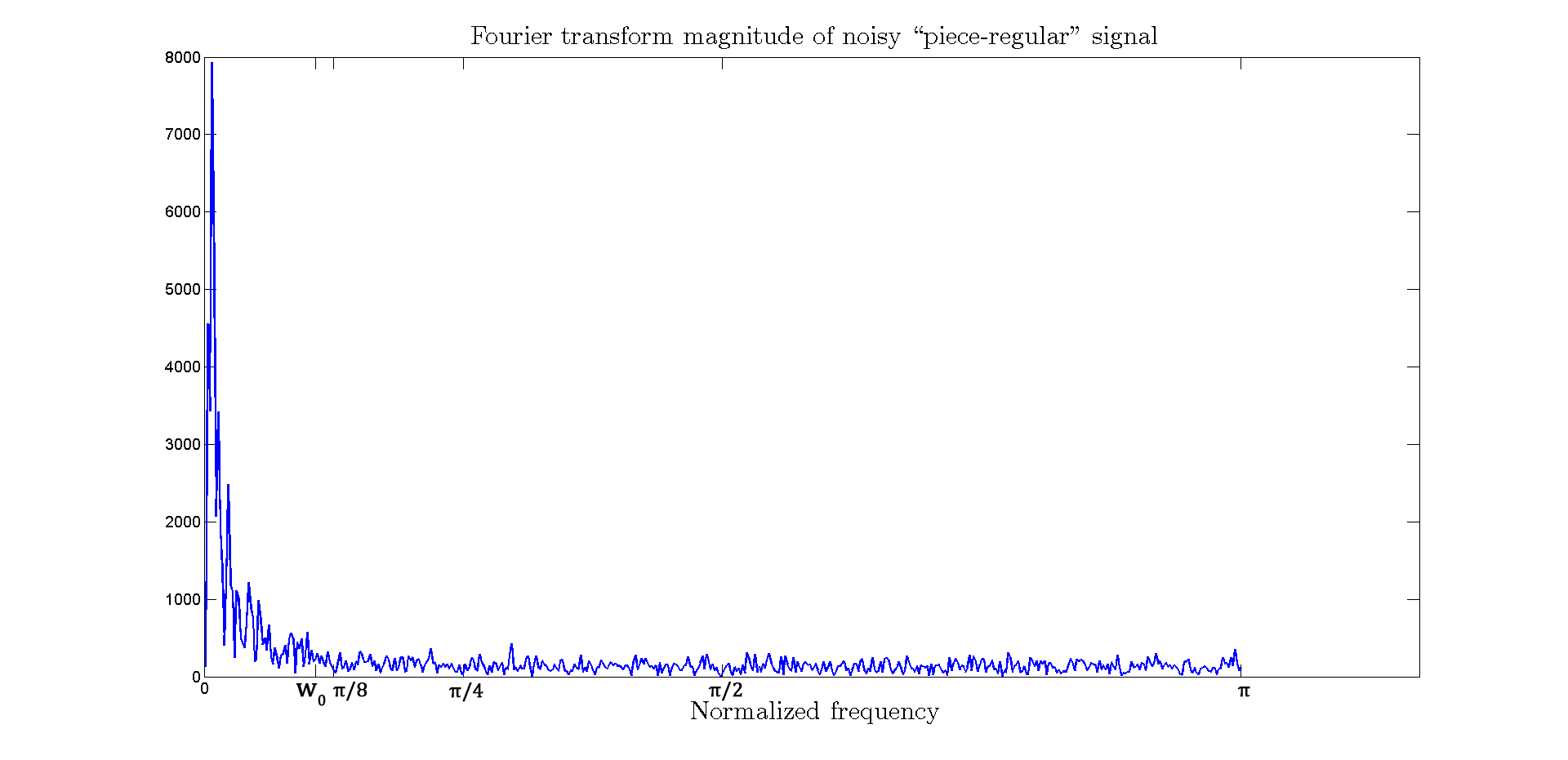
Fig. 5
Epigraph set
based threshold selection is compared with wavelet denoising methods
used in MATLAB [2, 3, 4, 5]. The "piece-regular" signal shown in Fig. 1
is corrupted by a zero mean Gaussian noise with of
the
maximum amplitude of the original signal. The signal is restored using
PES-L1 with pyramid structure, PES-L1 with wavelet, MATLAB's wavelet
multivariate denoising algorithm [3, 4], MATLAB's soft-thresholding
denoising algorithm, and Peyre's denoising method. The denoised
signals using
PES-L1 with pyramid structure, PES-L1 with wavelet are shown in Fig. 4,
and 6, with SNR values equal to 18.53,
18.05, respectively. Results for other test
signals in MATLAB are presented in Tables in the paper above. These
results are obtained by averaging the SNR values after repeating the
simulations for 300 times. The SNR is calculated using: worigworigwrec.
The denoised "piece-regular" signal with PES-L1 using wavelet
decomposition is as follows:
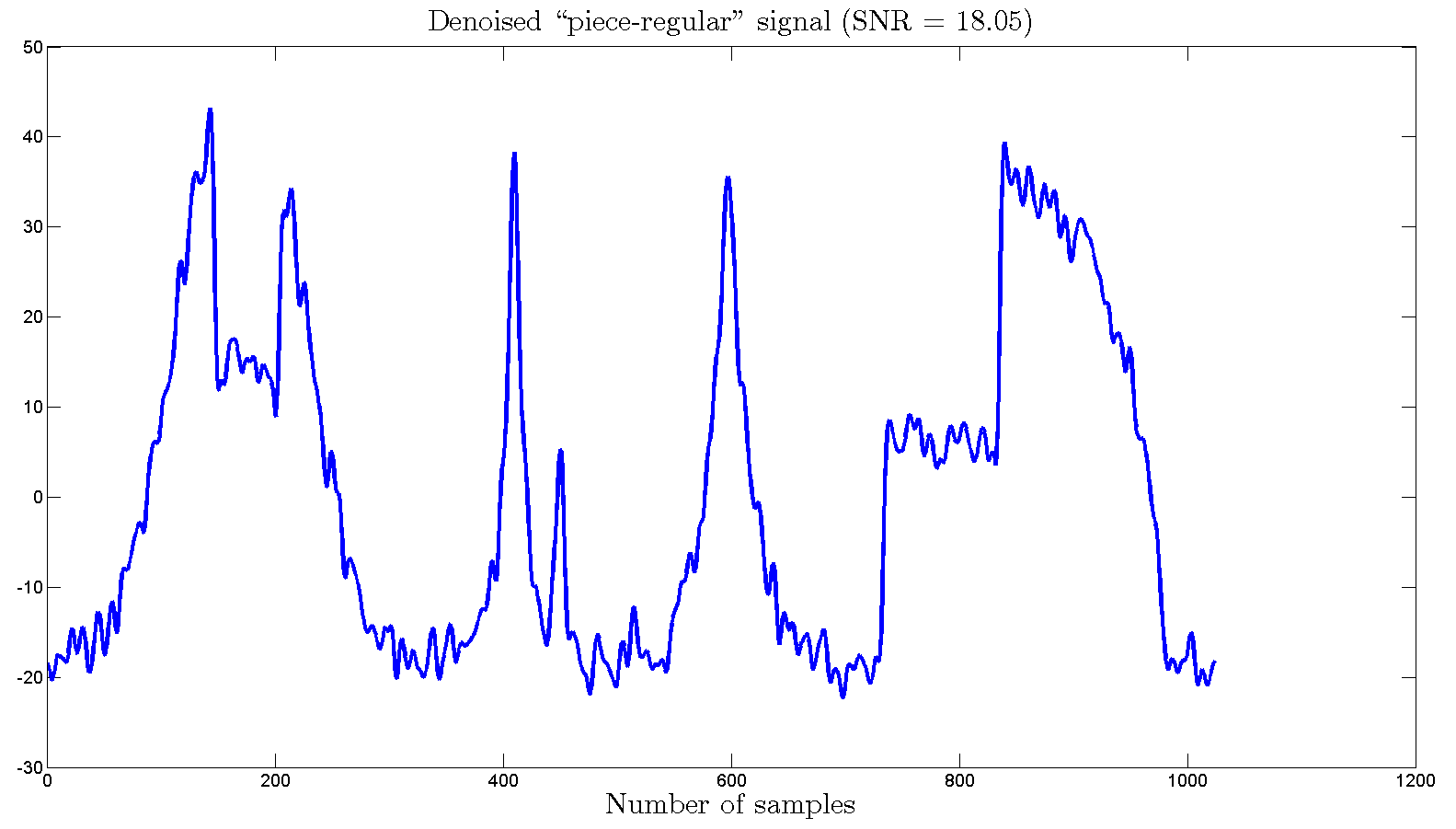
Fig. 6
Bibliography
[1]
S. Mallat and W.-L. Hwang, “Singularity detection and
processing
with wavelets,” Information Theory, IEEE Transactions on,
vol.
38, no. 2, pp. 617–643, Mar 1992.
[2] D. Donoho, “De-noising by soft-thresholding,”
Information Theory, IEEE Transactions on, vol. 41, no. 3, pp.
613–627, May 1995.
[3] M. Aminghafari, N. Cheze, and J.-M. Poggi, “Multivariate
denoising using wavelets and principal component analysis,”
Computational Statistics and Data Analysis, vol. 50, no. 9, pp. 2381
– 2398, 2006.
[4] P. J. Rousseeuw and K. V. Driessen, “A fast algorithm for
the
minimum covariance determinant estimator,” Technometrics,
vol.
41, no. 3, pp. 212–223, 1999.
[5] S. Chang, B. Yu, and M. Vetterli, “Adaptive wavelet
thresholding for image denoising and compression,” IEEE
Transactions on Image Processing, vol. 9, no. 9, pp.
1532–1546,
Sep 2000.
[6] D. L. Donoho and I. M. Johnstone, “Adapting to unknown
smoothness via wavelet shrinkage,” Journal of the American
Statistical Association, vol. 90, no. 432, pp. 1200–1224,
1995.
[Online]. Available:
http://amstat.tandfonline.com/doi/abs/10.1080/01621459.1995.10476626
[7] G. Chierchia, N. Pustelnik, J.-C. Pesquet, and B. Pesquet-Popescu,
“An epigraphical convex optimization approach for
multicomponent
image restoration using non-local structure tensor,” in IEEE
ICASSP, 2013, 2013, pp. 1359–1363.
[8] A. E. Cetin, A. Bozkurt, O. Gunay, Y. H. Habiboglu, K. Kose, I.
Onaran, R. A. Sevimli, and M. Tofighi, “Projections onto
convex
sets (POCS) based optimization by lifting,” IEEE GlobalSIP,
Austin, Texas, USA, 2013.
[9] K. Kose, V. Cevher, and A. Cetin, “Filtered variation
method
for denoising and sparse signal processing,” in 2012 IEEE
International Conference on Acoustics, Speech and Signal Processing
(ICASSP), March 2012, pp. 3329–3332.
[10] G. Chierchia, N. Pustelnik, J.-C. Pesquet, and B. Pesquet-Popescu,
“Epigraphical projection and proximal tools for solving
constrained convex optimization problems: Part i,” Arxiv,
CoRR,
vol. abs/1210.5844, 2012.
[11] J. Duchi, S. Shalev-Shwartz, Y. Singer, and T. Chandra,
“Efficient projections onto the l1-ball for learning in high
dimensions,” in Proceedings of the 25th International
Conference
on Machine Learning, ser. ICML ’08. New York, NY, USA: ACM,
2008,
pp. 272–279.
[12] R. Baraniuk, “Compressive sensing [lecture
notes],”
IEEE Signal Processing Magazine, vol. 24, no. 4, pp. 118–121,
2007.
[13] J. Fowler, “The redundant discrete wavelet transform and
additive noise,” Signal Processing Letters, IEEE, vol. 12,
no. 9,
pp. 629–632, Sept 2005.
|